notdecidedyet

한줄평 : 2017 Attention Is All You Need 에서 사용한 Absolute Positional Embedding의 문제를 보완한 Positional Embedding 방법들을 살펴보고, Rotary Positional Embedding을 제안한다.

1. Introduction.

PLM(Pretrained Language Model)은 Self Attention 아키텍쳐에서 위치에 구애받지 않는 것으로 나타난다. 따라서 위치 정보를 인코딩 하기 위해 다양한 접근이 제안되었다.

- Absolute Positional Embedding : Attention is All You Need(2017), Gehring(2017), Devlin(2019), Lan(2020)...등등

- Relative Positional Embedding : Raffel[2020], Ke[2020], He[2020], Huang[2020] 등등

(유명한 relative Positional Embedding사용한 논문으로는 ALiBi가 있다.)

위 방법들은 효과적이나 일반적으로 위치 정보를 컨텍스트에 추가하기 때문에 linear self-attention 구조에서는 적합하지 않다.

이 논문에서는 RoPE라는 방법을 소개한다. RoPE는 회전 행렬로 절대 위치를 인코딩하는 동시에 Self attention 수식에 상대적인 정보도 주입한다. 해당 방법론은 시퀀스 길이에 유연하며, 상대적 거리 증가에 따른 토큰 간 의존성 감소, 등 기존 방법보다 좋은 특성들이 많다.

2. BackGround and Related Work

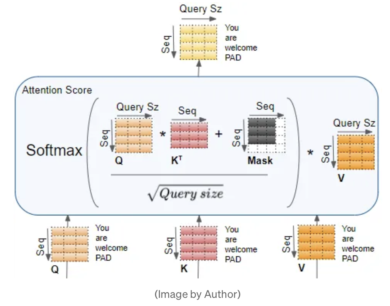
2.1 Preliminary - 일반적인 attention이 어떻게 계산되는지 설명

2.2 Absolute Positional Embedding - Sinosoid Embedding - Transformer(2017)의 positional embedding을 설명

2.3 Relative Positional Embedding - Attention구조에서 Relative Positional Embedding이 어떻게 수학적으로 흘러가는지 표현

3. Proposed Approach

Transformer의 self-attention에서는 query와 key 벡터 사이의 내적을 통해 토큰 간의 관계를 파악한다. 내적 연산에 relative position 정보를 자연스럽게 반영하기 위해, query 벡터 q_m과 key 벡터 k_n의 내적이 두 토큰의 단어 임베딩 x_m, x_n과 상대 위치인 m-n에 의해서만 결정되어야 한다고 말한다.

여기서  <,>은 내적 연산을 나타내고, g는 오직 두 토큰의 단어 임베딩과 그들 간의 상대 위치 m-n에 의해서 결정되는 함수이다.

이런 조건을 만족하는 fq와 fk를 찾는 것이 RoPE의 목표이다. (여기서 f는 embedding을 의미함 -> RoPE)

해당 방법을 유도하는 것은 (3.4.1 Derivation of RoPE under 2d)에 있으니 관심있으신 분들은 찾아보는 것을 추천한다.

(주인장은 시간이 주어질 때 뜯고 씹고 맛보기 위해 남겨 놓겠다.

기존 방법들이 주로 position embedding을 단어 임베딩에 직접 더하는 형태였다면, RoPE는 position 정보를 내적 연산에 자연스럽게 녹여내고자 한다.

2D 공간에서 위 수식을 만족하는 것은 아래 식처럼 나타낼 수 있다.

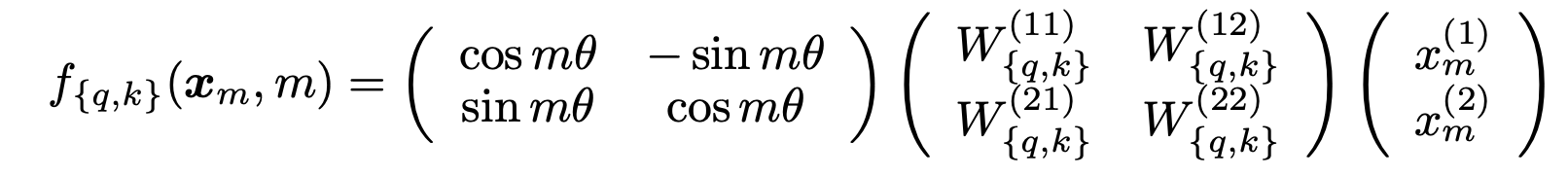
젊을적 수학을 쫌 하셨다 하신 분들 께서는 어디서 익숙한데 라는 느낌을 받을 것이다.

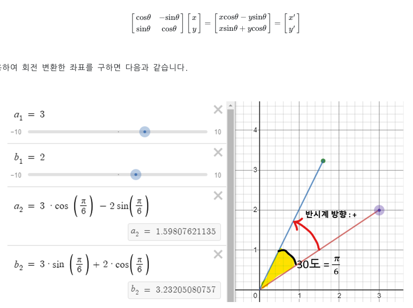
회전 변환과 매우 흡사하게 생겼다. 아래 그림은 김진솔 님의 블로그에서 퍼온 것인데, 2차원 벡터에서 세타만큼 회전할 때 사용하는 수식과 매우 흡사하다. 다만 다른점이라고는 learning 하는 파라미터가 중간에 들어갔다 정도이다.

너무 두서없이 작성하여 여기서 한번 정리하고 넘어가자.

g라는 함수는 단순하게 단어 임베딩 벡터를 위치 인덱스의 각도의 곱만큼 회전하기만 된다는 직관적인 해석이 가능하다.

D 공간에서는 그럼 어떻게 할까?

논문에 의하면 위와같이 한다고 한다. 수학은 처음에는 어려워 보이나 핵심을 알면 간단하다. 하나씩 살펴보자

2D상황에서 찾은 방법을 word dim에 적용하고 싶은거다. 2d에 적용할때 2개의 데이터 쌍으로 벡터 회전을 하였으니 여기서는 d개의 차원을 2로 나누어 d/2개 쌍으로 묶어서 회전을 할 수 있지 않을까 라고 생각한 것으로 보인다.

아래 그림으로 보면 더 명확하다. 

왼쪽 첫번째 단어 Enhanced는 d의 차원을 갖고 있고, 이를 d/2 쌍으로 나누어 position인 1번 포지션에 맞게 회전을 시킨다.

그래서 구현은 어떻게 하는건데?

위에서 언급한 Matrix는 너무 Sparse하여 계산을 하는데 무리가 있다.

논문에서는 효율적으로 계산하는 법을 제안한다.

m번째 단어가 있다고 할때 m단어가 갖는 dim을 기반으로 계산을 하면 아래와 같고, 이를 바탕으로 구현을 하면 되겠다.

class RotaryPositionalEmbeddings(nn.Module):
    def __init__(self, dim, max_position_embeddings=2048, base=10000, device=None, scaling_factor=1.0):
        super().__init__()
        self.dim = dim
        self.max_position_embeddings = max_position_embeddings
        self.device=device
        self.scaling_factor = scaling_factor
        self.base = base
        inv_freq = 1.0 / (self.base ** (torch.arange(0, self.dim, 2, dtype=torch.int64).float().to(device) / self.dim))  # max_position embedding // 2
        self.register_buffer("inv_freq", inv_freq, persistent=False)

        self._set_cos_sin_cache(
            seq_len=max_position_embeddings, device=self.inv_freq.device, dtype=torch.get_default_dtype()
        )

    def _set_cos_sin_cache(self, seq_len, device, dtype):
        self.max_seq_len_cached = seq_len
        t = torch.arange(self.max_seq_len_cached, device=device, dtype=torch.int64).type_as(self.inv_freq)
        t = t / self.scaling_factor
        freqs = torch.outer(t, self.inv_freq)
        emb = torch.cat((freqs, freqs), dim=-1)
        self.register_buffer("cos_cached", emb.cos().to(dtype), persistent=False)
        self.register_buffer("sin_cached", emb.sin().to(dtype), persistent=False)

    @torch.no_grad()
    def forward(self, x, seq_len=None):
        # x: [bs, num_attention_heads, seq_len, head_size]
        if seq_len > self.max_seq_len_cached:
            self._set_cos_sin_cache(seq_len=seq_len, device=x.device, dtype=x.dtype)

        return (
            self.cos_cached[:seq_len].to(dtype=x.dtype),
            self.sin_cached[:seq_len].to(dtype=x.dtype),
        )

    def apply_rope(self, x: torch.Tensor, cos: torch.Tensor, sin: torch.Tensor, position_ids, unsqueeze_dim=1) -> torch.Tensor:
        cos = cos[position_ids].unsqueeze(unsqueeze_dim)
        sin = sin[position_ids].unsqueeze(unsqueeze_dim)
        x1 = x[..., : x.shape[-1] // 2] 
        x2 = x[..., x.shape[-1] // 2 :] 
        rotated = torch.cat((-x2, x1), dim=-1) 
        roped = (x * cos) + (rotated * sin)
        return roped.to(dtype=x.dtype)

    @property
    def sin_cached(self):
        return self._sin_cached

    @property
    def cos_cached(self):
        return self._cos_cached

해당 로터리 임베딩은 attention구간에서 발생한다.

이 논문에서 처음부터 구체화 하고자 하는 것과, 논문의 시작과 끝까지 attention에 있어서 positional embedding의 역할에 대해서 포커스를 맞추었고, 식 16을 살펴보면 query key attention구간에서 R을 정의하고 있다. 따라서 코드도 당연하게 forward부분에서 발생한다.

class Attention(nn.Moduel):
	def __init__(self, ...):
    	...
        self.rotary_emb = RotaryPositionalEmbeddings(
            head_dim,
            max_position_embeddings=config.max_position_embeddings,
            device=config.device,
            base=config.rope_theta,
        )

		...
    def forward(self, ...):
        kv_seq_len = keys.shape[-2]
        cos, sin = self.rotary_emb(values, seq_len=kv_seq_len)
        queries = self.rotary_emb.apply_rope(queries, cos, sin, position_ids)
        keys = self.rotary_emb.apply_rope(keys, cos, sin, position_ids)

GQA에 들어가기에 앞서, 

어텐션에 무엇이 존재하는지 알아보자.

Attention Is All You Need에 언급되었던 Multi Head Attention (2017)

- AI산업 전설의 시작이 되는 컨셉으로, 이후에 vision, anomaly, recommend, audio 모든 영역으로 퍼져나감

- 단점 : 계산의 bottleneck 현상이 발생할 수 있고, computational resource를 매우 많이 잡아먹는 작업이다.

KV cached Attention 

- Inference시에 AutoRegressive하게 추론을 진행

- 위 그림에서, without cache 버전을 살펴보면 매 Inferece시점에서 과거에 계산한 QK를 다시 반복해서 수행해야 한다. (이미 과거에 추론한 데이터는 바꿀 수 없는데 말이다)

- 따라서 아래 제안한 with cache버전은, 이미 지나간 key는 계산하지 않고 저장해둔다. query에서는 해당 시점의 쿼리만 가져와서 계산을 해준다

- 단점 : key들을 어디 저장을 해두어야 하는데, 이로인해 seq길이가 길어지면 메모리에 저장되는 용량이 커져서 문제가 된다.

Multi Query Attention : Fast Transformer Decoding : One Write-Head is All You Need(2019, google)

- K,V에는 MultiHead를 적용하지 않고, Query에만 적용한다.

- 장점 : 이로인해 퍼포먼스는 증가하고, 모델의 성능은 아주 적게 감소하였다.

- 추론에서 11배 빠른 처리량과, 30%더 낮은 대기시간을 얻었다.

- 단점 : Multi Head Attention에 비해 성능이 저하될 위험이 있고, 학습이 불안정하다.

GQA: Training Generalized Multi-Query Transformer Models from Multi-Head Checkpoints

가운데 있는 그림이 GQA로, MHA와 MQA을 섞어 놓은 버전으로 생각하면 좋다.

연구 결과

• Multi-head attention(MHA)이 있는 언어 모델 체크포인트를 multi-query attention (MQA)를 사용하도록 업트레이닝하는 방법을 제안. 빠른 inference와 고품질 체크포인트를 얻는 비용 방법
• Grouped-query attention (GQA)이라는 새로운 방법을 제안. GQA는 query head의 하위 그룹당 하나의 key와 value head를 사용하여 MHA와 MQA를 보완. 업트레이닝된 GQA는 MQA만큼 빠르면서도 MHA에 가까운 품질을 달성할 수 있다.

import torch
import torch.nn.functional as F
from einops import rearrange, einsum

# [batch, seq_len, num_heads, head_dim]
query = torch.randn(1, 256, 8, 64)
key = torch.randn(1, 256, 2, 64)
value = torch.randn(1, 256, 2, 64)

# number of heads in one group, in this example 2 kv_heads
# -> it will be 2 groups of size 4 each
num_head_groups = query.shape[2] // key.shape[2]   # 8 // 2 -> 4
scale = query.size(-1)**0.5

# swap seq_len with num_heads to accelerate computations
query = rearrange(query, 'b n h d -> b h n d')
key = rearrange(key, 'b s h d -> b h s d')
value = rearrange(value, 'b s h d -> b h s d')

# split query num_heads in group by introducing additional 'g' dimension
query = rearrange(query, 'b (h g) n d -> b g h n d', g=num_head_groups)

# calculate attention scores and sum over the groupb dim to perform averaging
scores = einsum(query, key, 'b g h n d, b h s d -> b h n s')  # g는 broadcasting되어 계산고, average됨
# scores[b, h, n, s] = Σ(query[b, g, h, n, d] * key_broadcasted[b, g, h, s, d])
# reference of einsum https://haystar.tistory.com/93

attention = F.softmax(scores / scale, dim=-1)

out = einsum(attention, value, 'b h n s, b h s d -> b h n d')

out = rearrange(out, 'b h n d -> b n h d')

https://arxiv.org/pdf/2305.13245

https://medium.com/@joaolages/kv-caching-explained-276520203249

https://moon-walker.medium.com/long-context로-인한-large-kv-cache의-문제점과-해결-방안-part-i-kv-cache의-메모리-요구량-025f3d5dea93

https://r4j4n.github.io/blogs/posts/kv/

https://medium.com/@plienhar/llm-inference-series-4-kv-caching-a-deeper-look-4ba9a77746c8

https://medium.com/@maxshapp/grouped-query-attention-gqa-explained-with-code-e56ee2a1df5a

ASR SOTA모델 중 하나인 Wav2vec2 논문을 살펴보며, CodeBook, Quantization이라는 개념이 나오고, 잘 와닿지 않아 정리해본다.

왜... 왜 이산화를 해????? 정보가 많이 사라질텐데..?

이산화를 하는 이유는 인간이 발음할 수 있는 음소의 수가 한정되어 있기에 CodeBook을 사용한다고 한다

(물론, Continuous -> Discrete화 -> Continuous 하여 사용하는 것만은 아니다.)

(...모델 경량화 할 때 사용된다고 한다.)

(...GumbleSoftmax를 찾아보면 좋겠다.)

(...Continuous -> Discrete 화 하면, 코드 관점에서는 torch graph가 깨지고, 학문적 관점에서는 샘플링을 하는 것과 같기에 reparameterize trick과 같은것이 필요하다. -> 이것을 gumbleSoftmax로 풀어냄)

Feature Extracted된 부분이 Encoder 및 CodeBook으로 따로 흘러가며, 나중에 Concatenate을 하게 된다.

그렇다면 CodeBook은 어떻게 진행될까?

구체적으로 코드와 같이 살펴보자

wav2vec2를 기준으로 설명하자면

## shape들 ##

input_mfcc.shape = [bs, seq_len, feature]                            # wav -> mfcc 변환
input_mfcc_cnn.shape = [bs, seq_len, cnn_feature]           # mfcc -> cnn encoder로 특징 추출

input data가 mfcc 및 cnn으로 위와같이 변환된다.

이때 input_mfcc_cnn데이터가 FeatureExtractor(Masking 처리된 부분)과 CodeBook으로 흘러가게 된다.

여기서는 CodeBook부분만 살펴보자.

추후 GumbleSoftMax에 대해서 다루겠다.. 이만...

source code

https://github.com/HarunoriKawano/Wav2vec2.0

gumble softmax

https://data-newbie.tistory.com/263

https://kaen2891.tistory.com/81